딥러닝 기반의 쌍축선 연료 소모량 예측 연구

This is an Open-Access article distributed under the terms of the Creative Commons Attribution Non-Commercial License(http://creativecommons.org/licenses/by-nc/3.0) which permits unrestricted non-commercial use, distribution, and reproduction in any medium, provided the original work is properly cited.
Abstract
With growing pressure from the International Maritime Organization (IMO) to reach net-zero emissions by 2050, accurate prediction of ship Fuel Oil Consumption (FOC) has become increasingly important. Although numerous deep learning-based FOC prediction models have been proposed, studies targeting twin-screw ships remain scarce. In this paper, we propose a dual-branch deep learning architecture for multi-step FOC prediction of twin-screw ships, designed to capture the distinct operational characteristics of the port and starboard propulsion shafts. Each branch independently encodes feature-axis relationships using a Multi-Layer Perceptron (MLP) encoder and temporal patterns using a Gated Recurrent Unit (GRU) encoder. A Squeeze-and-Excitation (SE) block is employed to adaptively fuse the encoded representations, and an autoregressive GRU decoder then generates multi-step FOC predictions. The model is trained on five months of operational data from a RO-RO passenger ship navigating the Gunsan–Shidao route, supplemented with wave data from the Copernicus Marine Environment Monitoring Service (CMEMS). Experiments under various prediction conditions demonstrate that the proposed model consistently outperforms nine baseline models, including LSTM, GRU, transformer variants, and recent hybrid architectures, across the RMSE, MAE, and MAPE metrics.
Keywords:
Fuel oil consumption prediction, Twin-screw ship, Deep learning, Copernicus marine environment monitoring service, Gated recurrent unit키워드:
연료 소모량 예측, 쌍축선, 딥러닝, 코페르니쿠스 해양환경 모니터링 서비스, 게이트 순환 유닛1. 서 론
전 세계 무역의 80% 이상이 해상 운송을 통해 이루어지며, 이는 세계 경제 발전의 기반이 된다(UNCTAD, 2022). 해상 운송으로 발생하는 온실가스 배출량은 2012년 2.76%에서 2018년 2.89%로 증가하였고(IMO, 2020), 2022년 해운 산업은 약 7억 6백만 톤의 이산화탄소를 배출한 것으로 나타났다(Li et al., 2024). 이러한 추세가 지속될 경우, 2050년까지 이산화탄소 배출량이 최대 250%까지 증가할 것으로 전망된다(Roy and Chakraborty, 2025). IMO(국제해사기구, International Maritime Organization)는 단기, 중기, 장기적으로 각각 2030년까지 최소 30% 감소, 2040년까지 최소 70% 감소, 2050년까지 순배출량 제로 달성을 목표로 하며, 해상 운송의 효율성을 높이고 온실가스 배출량을 줄이기 위한 전략을 추진하고 있다(IMO, 2025).
해양 부문에서 에너지 효율성 개선은 연료 소비 절감과 직결되며, 이는 선박의 온실가스 배출량 감소에 직접적인 영향을 미친다. 이에 따라 연료 소모량 예측에 대한 연구가 활발히 진행되어 왔다. Gkerekos et al. (2019), Zhou et al. (2023), Yuksel et al. (2023), Fan et al. (2024)는 linear regression(LR), decision tree(DT), random forest(RF), support vector regression(SVR), k-nearest neighbors(KNN), artificial neural network(ANN) 등을 포함한 머신러닝 알고리즘을 비교 및 분석하였다. Lee et al. (2021)은 데이터 특성에 따라 deep feed-forward neural network(DFN) 구조를 변경한 모델을 제안하였고, Chen et al. (2024)는 ensemble empirical model decomposition(EEMD) 방법과 long short-term memory(LSTM)을 결합한 EEMD-LSTM 모델을 활용한 단기 다단계 예측 모델을 구축하였다. 제안된 모델은 30-60단계 구간에서 높은 정확도와 안정적인 성능을 보였다. 또한 Zhong et al. (2026)은 residual sparse graph convolutional network(ResGCN)와 improved LSTM(iLSTM)을 결합한 하이브리드 예측 프레임워크를 제안하였고, Song et al. (2025)는 temporal convolutional network(TCN), bidirectional gated recurrent units(BiGRU), attention을 결합한 병렬 구조의 하이브리드 예측 프레임워크를 제안함으로써 선박 운항 및 해양 기상 특성 간의 상호작용으로 인한 시공간적 의존성을 포착하지 못하는 어려움을 해결하였다. 이 밖에도 머신러닝 및 딥러닝 알고리즘을 활용한 연구가 다수 진행되어 왔으나, 대부분 단일 추진 선박을 대상으로 한정되어 있다.
본 연구는 연료 소모량 예측 연구가 충분히 이루어지지 않은 쌍축선에 주목한다. 쌍축선은 이중 추진기와 방향타를 탑재한 선박으로, 좌현과 우현에 각각 위치하는 추진기를 port와 starboard로 구분한다. 단일 추진기 고장 시에도 운항 지속이 가능하여 운항 안정성 측면에서 강점을 가진다. 쌍축선을 대상으로 한 기존 연구는 주로 유체역학적 저항 및 자항 성능 분석에 집중되어 왔으며(Kim et al., 2025; Gaggero and Martinelli, 2023), 실제 운항 데이터를 활용한 연료 소모량 예측 연구는 현재까지 거의 이루어진 바가 없다. 특히 이중 추진기가 설계상 동일한 구조를 가지더라도 마모 정도나 환경적 요인에 의해 다른 운항 패턴을 보일 수 있어, 본 연구에서는 각 추진기의 운항 특성 차이를 반영한 딥러닝 기반의 연료 소모량 예측 모델을 제안한다. 또한 다단계 시계열 예측은 예측 기간이 길어질수록 오차가 누적되어 성능이 저하되는 것으로 알려져 있다. 이에 따라 다양한 입력 및 출력 시퀀스 길이의 조합에 대한 실험을 진행하여 성능이 유지되는 구간을 검토하고자 한다.
본 연구의 구성은 다음과 같다. 2장에서는 제안 모델 및 방법을 살펴보고, 3장에서는 제안 모델과 비교 모델에 대한 실험을 진행하여 성능 평가 결과를 확인한다. 마지막으로, 4장에서는 본 연구에서 제시한 결과를 요약 및 정리한다.
2. 제안 모델 및 방법
본 연구에서 제안한 방법론은 Fig. 1과 같다. 먼저 수집된 선박 운항 데이터와 해양 기상 데이터를 통합하고, 전처리 작업을 수행한다. 이후 쌍축선의 port와 starboard 추진기 데이터를 독립된 입력으로 구성하며, 각 추진기의 운항 특성을 반영한 딥러닝 기반 모델 Dual MLP-GRU with SE를 제안하여 연료 소모량을 예측한다.
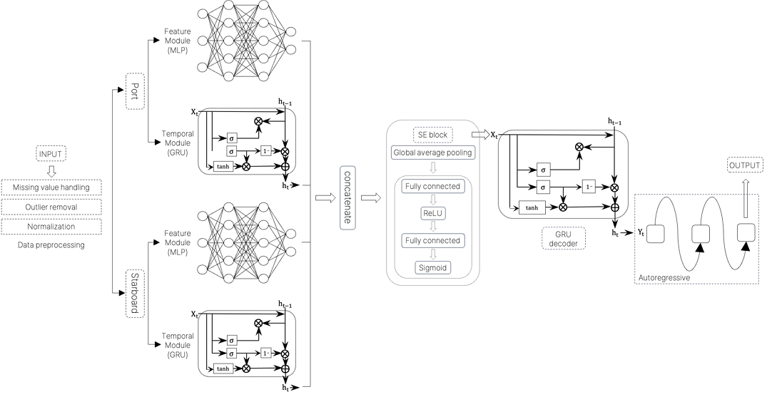
Overview of the Dual MLP-GRU with SE(proposed model)
2.1 선박 데이터
본 연구에서 사용한 대상 선박은 Table 1, Fig. 2와 같이 쌍축 추진 방식의 Roll on–Roll off(RO-RO) 여객선이다. 해당 선박은 화물과 여객을 동시에 운송하는 선종으로, IMO의 넷제로 프레임워크가 규제 대상 범위를 소형 선박까지 확대하고 있다는 점에서 해당 선박으로 선정하였다. 또한, 중국 석도와 대한민국 군산을 오가는 고정된 항로를 운항하는 특성상 항로 조건이 비교적 일정하여 예측 모델의 성능 평가에 적합한 환경을 제공할 수 있다.

Vessel specification
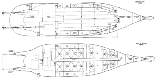
Twin-screw ship
2.2 데이터 수집
2025년 10월 2일부터 2026년 3월 7일까지 약 5개월 간의 선박 운항 데이터와 해양 기상 데이터를 수집하였다. 선박 운항 데이터는 Fig. 3과 같이 대한민국 군산과 중국 석도를 오가는 선박으로부터 수집된 10분 간격의 항해 및 엔진 정보로 구성된다. 해양 기상 데이터는 선박 센서 데이터의 위경도를 기반으로 Copernicus marine environment monitoring service(CMEMS)로부터 3시간 간격의 파랑 데이터를 수집하였고, 이 중 significant wave height의 분포 시각화는 Fig. 4와 같다. 총 12,178행의 데이터를 활용하였고, 항해 데이터 일부는 Table 2와 같다.
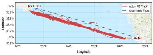
Ship route between GUNSAN and SHIDAO
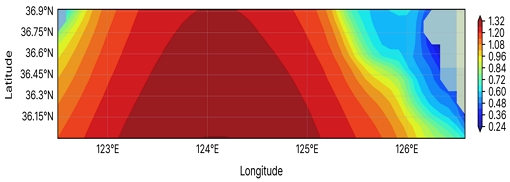
Spatial distribution of significant wave height
Summary statistics of features
2.3 데이터 전처리 및 정제
선박 운항 데이터는 수집 과정에서 센서 오류로 인한 이상치 및 기록 불일치 등이 존재할 가능성이 있으므로, 데이터 전처리는 데이터의 정확성과 일관성을 보장하는 데 매우 중요하다. 먼저, 문자열 이상치(-, ., .., NaN, 99999)와 센서 측정 오류(예: 6과 8, 2와 5 등을 오인식)를 제거하였다. 다음으로, 센서 데이터에서 누적 값으로 기록된 port와 starboard의 연료 소모량 값을 10분 단위로 차분하여 구간별 연료 소모량을 산출하였고, 이 과정에서 물리적으로 불가능한 값은 제외하였다. 또한 10분 간격의 항해 데이터와 3시간 간격의 해양 기상 데이터의 샘플링 간격을 10분으로 통일하였다. 더불어 입력 및 출력 시퀀스를 구성할 때 결측 값이나 시간 간격이 10분으로 일정하지 않은 경우는 해당 시퀀스 전체를 제외함으로써 데이터의 연속성을 확보하였다.
이후 전처리된 데이터는 훈련 및 테스트 데이터셋을 8:2 비율로 분리하였다. Fig. 5와 같이 TimeSeriesSplit cross validation을 적용하여 훈련 데이터셋은 검증 데이터셋보다 과거 시점의 데이터가 활용되었으며, n_splits을 5로 설정하여 5번의 반복으로 cross validation을 진행하였다. 일반적으로 split은 시간의 순서를 고려하여 매 반복마다 학습 구간이 누적되어 확장되는 방식으로 구성된다. 테스트 데이터셋은 cross validation에 포함되지 않고, 5번의 독립적으로 학습된 모델을 각각 평가하는 데에 동일하게 사용되었다.
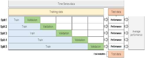
Structure of TimeSeriesSplit cross validation
분할된 데이터는 모든 변수가 동일한 척도를 갖도록 z-score 정규화를 적용하였다. 각 변수 x에 대해 평균 μ와 표준편차 σ를 산출하였으며, 표준화된 변수 z는 식 (1)과 같이 구할 수 있다.
| (1) |
또한 Table 2의 기존 변수들을 활용하여 보다 정밀하게 학습될 수 있도록 파생 변수를 생성하였다. 기존의 풍향 및 파향 데이터를 선박의 heading 기준 상대값으로 변환하였고, relative wind angle(상대 풍향)과 relative wave angle(상대 파향)은 식 (2), (3)과 같다.
| (2) |
| (3) |
2.4 Encoder
Multi-layer perceptron(MLP)는 Fig. 6과 같이 input layer(입력층), 하나 이상의 hidden layer(은닉층), output layer(출력층)으로 구성된 fully-connected(완전연결) 형태이다. 각 층의 뉴런은 이전 층의 모든 뉴런과 연결되며, 선형 변환과 비선형 활성화 함수의 조합을 통해 입력 데이터의 복잡한 관계를 학습한다.
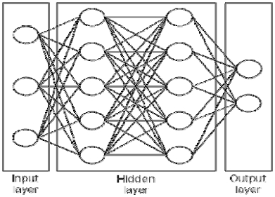
Structure of MLP
본 연구에서 port와 starboard 각각에 MLP를 적용함으로써, 각 시점에서의 입력변수 간 비선형 관계를 학습하는 feature encoder로 활용한다.
Gated recurrent unit(GRU)는 LSTM의 복잡한 구조를 단순화한 recurrent neural network(RNN) 계열의 변형 모델이다. 별도의 cell state를 포함하지 않으며, update gate와 reset gate로 구성된다. update gate는 이전 정보와 현재 정보를 얼마나 반영할지 결정하고, reset gate는 이전 정보를 얼마나 잊을지를 결정한다. Reset gate의 출력과 현재 정보를 결합하여 후보 은닉 상태가 산출되며, 최종 은닉 상태는 update gate에 의해 이전 정보와 후보 은닉 상태를 가중 결합하여 결정된다. 산출된 은닉 상태는 다음 시점으로 전달되는 동시에 선형 변환을 거쳐 최종 출력으로 산출된다(Cho et al., 2014). GRU의 연산은 식 (4)~(8)과 같다.
| (4) |
| (5) |
| (6) |
| (7) |
| (8) |
본 연구에서는 feature module과 마찬가지로 port와 starboard에 각각 독립적인 GRU를 적용함으로써, 과거 관측 구간 내 시계열의 시간적 패턴을 학습하는 temporal encoder로 활용한다.
또한 두 축의 MLP와 GRU는 서로 다른 파라미터를 가지며, 파라미터를 공유하지 않고 각 축의 특성을 독립적으로 학습한다.
2.5 SE block & decoder
Squeeze & Excitation(SE) block은 Fig. 7과 같이 여러 표현에 대한 중요도를 학습하여 유용한 정보는 선택적으로 강조하고 불필요한 정보는 억제한다(Hu et al., 2018). Port와 starboard 각각에 대해 MLP encoder의 출력 값과 GRU encoder의 최종 은닉 상태를 하나의 표현 집합 로 SE block을 적용한다.
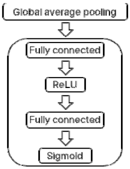
Structure of SE block
SE block은 식 (9)와 같이 입력 표현을 α 방향으로 평균하여 요약 통계량 z를 계산한다. 이후 식 (10), (11)을 통해 완전연결-ReLU-완전연결-sigmoid를 거쳐 가중치벡터 g로 변환한 뒤, 산출한 g를 원래 표현에 곱한다. 본 연구에서는 해당 연산을 특징 축에 대해서만 적용하여 최종 재조정된 표현인 을 얻는다. 시간 축은 SE block 연산에 포함되지 않으며, 개별 시점의 정보는 그대로 보존된다(Jin et al., 2022).
| (9) |
| (10) |
| (11) |
산출된 는 하나의 벡터로 decoder의 context vector c를 구성하며, 식 (12)와 같다. 이는 식 (13), (14)를 통해 decoder의 초기 은닉 상태 h0과 초기 입력 으로 각각 변환된다.
| (12) |
| (13) |
| (14) |
이후 이전 시점의 예측값을 다음 시점의 입력으로 사용하는 자기회귀 방식으로 연료 소모량을 순차적으로 예측한다.
2.6 성능 지표
선박의 연료 소모량 예측 모델의 안정성 및 성능을 평가하기 위해 세 가지 성능 평가 지표를 활용하였다.
Root mean squared error(RMSE)는 예측 오차를 제곱하여 평균한 뒤 제곱근을 취한 값으로, 오차의 크기를 실제값과 동일한 단위로 나타낸다. Mean absolute error(MAE)는 예측값과 실제 값 사이의 절대 오차 평균으로, RMSE에 비해 이상치의 영향을 덜 받는다. 마지막으로, mean absolute percentage error(MAPE)는 예측 오차를 실제값에 대한 백분율로 표현하여 데이터 범위에 무관하게 상대적 예측 정확도를 평가할 수 있다. 세 가지 성능 지표는 식 (15)~(17)과 같이 계산된다.
| (15) |
| (16) |
| (17) |
3. 예측 성능 평가 결과
본 장에서는 실험 설계 및 설정과 예측 모델 성능 평가에 대한 결과를 분석한다.
3.1 실험 설계 및 설정
제안된 모델의 성능을 검증하기 위해 본 논문에서는 총 9개의 모델과 비교하였다. RNN 및 MLP 계열의 LSTM(Hochreiter and Schmidhuber, 1997), GRU(Cho et al., 2014), TSMixer(Chen et al., 2023), 연료 소모량 예측 분야의 최신 모델인 TCFFA- GRU-Parallel(Hao et al., 2025)과 TSBG-Para(Song et al., 2025), transformer 계열의 transformer(Vaswani et al., 2017), informer(Zhou et al., 2021), reformer(Kitaev et al., 2020)와 convolutional neural network(CNN) 계열의 temporal convolutional network(TCN)(Bai et al., 2018)을 포함하였다.
하이퍼파라미터는 모델의 학습 과정을 제어하고, 모델의 성능에 큰 영향을 미친다. 제안 모델의 하이퍼파라미터 튜닝은 Table 3과 같이 탐색 범위를 설정하여 optuna로 하이퍼파라미터를 최적화하였다(Akiba et al., 2019). 비교 모델의 경우, 제안 모델에 맞게 동일한 범위로 탐색하였으며 제안 모델의 하이퍼파라미터 설정 값은 Table 4에 정리되어 있다. 아울러 모든 실험은 13th Gen Intel(R) Core(TM) i5-13400 프로세서와 32GB RAM을 탑재한 Window 11 환경에서 수행되었다.
Parameter ranges of all models for hyperparameter tuning
Hyperparameter settings of proposed model
3.2 예측 모델 성능 평가
본 연구는 딥러닝 기반의 연료 소모량 예측 모델인 Dual MLP-GRU with SE를 제안하였다. 예측 모델은 예측 시점 이전의 관측 구간을 설정하여 입력 시퀀스로 활용하고, 이를 기반으로 이후 시점에 대해 연료 소모량을 예측한다. 모델 성능 평가 지표는 RMSE, MAE, MAPE를 사용하였다.
Table 5와 Table 6은 각각 출력 시퀀스 길이 20분, 30분 조건에서 입력 시퀀스 길이 10~40분에 대해 평균 성능을 확인한 결과이다. 두 결과 모두 제안 모델이 모든 조건에서 가장 우수한 성능을 보였다. Table 5의 경우, 비교 모델 중 GRU, Transformer와 TSBG-Para가 상대적으로 우수한 성능을 보였다. 반면 Table 6의 경우, 두 모델의 성능이 크게 저하된 것을 확인할 수 있었고, TCN과 Reformer가 비교적 낮은 오차와 작은 표준편차를 유지하는 것으로 나타났다. 특히 GRU는 두 조건 모두 표준편차가 작아, 입력 및 출력 시퀀스 길이 조건이 달라지더라도 성능 변동이 크지 않은 안정적인 학습 경향을 보였다.
Overall performance comparison across all input-output length settings(input:10~40min, output: 20min)
Overall performance comparison across all input-output length settings(input:10~40min, output: 30min)
앞선 비교와 달리, Table 7은 출력 시퀀스 길이 조건을 구분하지 않고 전체 조합을 통합한 결과이다. 특히 비교 모델 중 가장 안정적인 성능을 보이는 GRU를 baseline(기준)으로 삼아 전체 8가지 조합에 대한 평균 성능과 GRU 대비 증감률을 함께 제시하였다. 그 결과, 제안 모델은 전 지표에서 GRU 대비 각각 RMSE 2.8%, MAE 5.0%, MAPE 4.4%로 개선된 성능을 보임을 확인할 수 있었다.
Overall performance comparison across all input-output length(baseline: GRU)
Fig. 8~10도 마찬가지로 출력 시퀀스 길이 조건을 구분하지 않고, 입력 시퀀스 길이 10~40분 구간에서의 모델별 평균 성능 추이를 지표별로 나타낸 결과이다. 제안 모델은 입력 시퀀스 길이 전 구간에서 가장 낮은 오차를 유지하였으며, 입력 시퀀스 길이가 짧을수록 비교 모델과의 차이가 뚜렷하게 나타났다. Transformer의 경우, 입력 시퀀스 길이 변화에 대해 상대적으로 민감하게 반응하는 것을 확인할 수 있다.
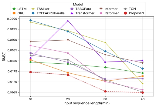
Overall RMSE comparison across all models by input sequence length
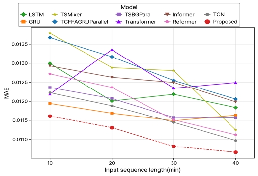
Overall MAE comparison across all models by input sequence length
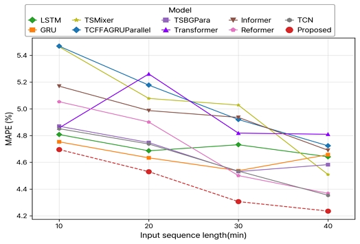
Overall MAPE comparison across all models by input sequence length
더불어 제안 모델의 dual 구조가 실제로 성능 향상에 기여하는지 검증하기 위해 port와 starboard 데이터를 하나로 통합한 single-branch 구조와 제안 모델의 비교 실험을 진행하였다. 이때 실험 설정은 제안 모델과 동일하게 설정되었으며, single-branch의 결과는 Table 8과 같다. Fig. 11~13을 보면, 입력 시퀀스 길이가 길어질수록 대체로 모델 간의 격차가 확대되는 것을 확인할 수 있는데, 이는 관측 기간이 길어질수록 port와 starboard 각각의 독립적인 인코딩 구조가 더 많은 시계열 정보를 활용할 수 있다고 해석할 수 있다.
Performance of the single-branch model (improvement rate of the proposed model over the single-branch model)
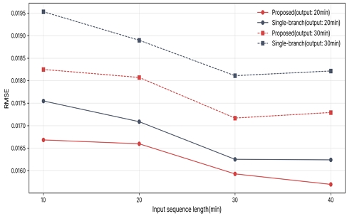
RMSE comparison between the single-branch and proposed model by input sequence length(output: 20 and 30 min)
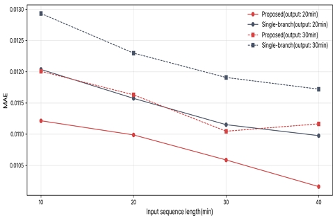
MAE comparison between the single-branch and proposed model by input sequence length(output: 20 and 30min)
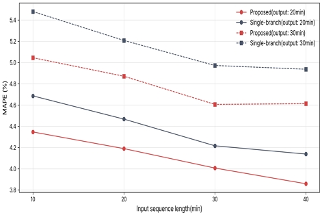
MAPE comparison between the single-branch and proposed model by input sequence length(output: 20 and 30min)
Fig. 14~15는 제안 모델의 예측값이 실제 연료 소모량의 변화 양상을 얼마나 정확히 반영하는지 확인하기 위해 실제값과 예측값을 비교한 결과이다. 출력 시퀀스 길이를 20분으로 고정하고 입력 시퀀스를 10~40분 구간의 모든 조건을 통합하여 시각화하였다. 전체적으로 제안 모델의 예측값은 연료 소모량이 급격히 증감하는 구간을 포함하여 실제값의 전반적인 변화 추이와 유사한 양상을 보였으며, 이는 큰 편차 없이 강건한 예측 성능을 유지함을 보여준다.
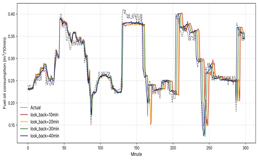
Actual and predicted fuel oil consumption(output: 20min)
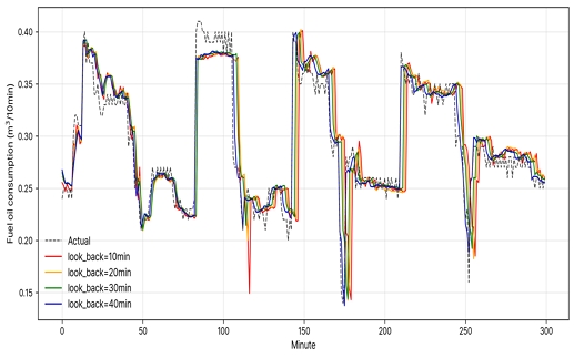
Actual and predicted fuel oil consumption(output: 30min)
Fig. 16은 SE block에서 산출된 가중치를 원래 입력변수 단위로 환산하여 변수별 상대적 가중치를 나타낸 결과이다. 상대 풍향과 상대 파향은 각 축에서 약 15~16%의 가중치를 보였으며, 그 다음으로 pitch가 약 8.5~9.3%의 가중치를 나타냈다. 이는 학습 과정에서 SE block이 선박의 저항 및 추진 효율과 관련된 특징을 상대적으로 크게 강조하였음을 보여준다.
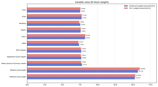
Variable-wise SE block weights
4. 결 론
본 연구는 쌍축선의 연료 소모량 예측을 위한 딥러닝 기반의 모델을 제안하였다. Port와 starboard 각 추진기의 운항 특성을 독립적으로 학습하기 위해 MLP와 GRU encoder를 병렬로 구조화하였으며, SE block을 통해 변수 간 관계 정보와 시간적 패턴 정보를 융합하였다. 이후 자기회귀 방식의 GRU decoder를 통해 다단계 연료 소모량을 순차적으로 예측하였다.
다양한 시퀀스 조건에서 9가지 비교 모델과의 성능 비교 결과, 제안 모델은 RMSE, MAE, MAPE 전 지표에서 가장 우수한 성능을 보였다. 또한 출력 시퀀스 길이를 고정한 상황에서 예측 시점 이전의 관측 구간 길이를 변화시키는 실험에서도 일관된 성능을 유지함으로써 제안 모델이 다양한 시퀀스 길이에서 강건한 예측 성능을 보임을 확인하였다. 아울러 port와 starboard를 하나로 통합한 모델과의 비교 실험을 통해, 제안 모델의 dual 구조가 실제로 성능 향상에 기여함을 확인하였다.
더불어 본 연구는 실제 선박 운항 데이터와 해양 기상 데이터를 통합하여 쌍축선의 연료 소모량 예측을 한 초기 연구로서 의의가 있다. 특히 단일 추진 선박에 집중되어 있는 기존 연구의 공백을 채우고, 쌍축선에 대한 데이터 기반 예측 연구의 가능성을 입증하였다. 또한 실제 해양 환경 요인인 파랑 데이터를 함께 결합함으로써 보다 현실적인 예측 환경을 구성하였다.
그러나 본 연구는 몇 가지 한계점을 가진다. 대한민국 군산과 중국 석도 간 왕복 항해 데이터를 항해 방향 및 계절 구분 없이 통합하여 학습에 활용하였기 때문에 실제 port와 starboard의 부하 패턴이 갖는 물리적 의미가 희석될 가능성이 있다. 또한 해양 환경 요인으로는 파랑 데이터만 수집함으로써 해류 및 조류 등 다양한 환경 요인을 반영하지 못하였다. 더불어 본 연구의 데이터는 10분 간격으로 수집되어, 이를 시간 및 일 단위로 환산할 경우, 활용 가능한 표본 수가 줄어들어 안정적인 학습이 어렵다. 향후 연구에서는 선박이 항해하는 방향 및 계절에 따라 데이터를 분리하여 진행할 것이며, port와 starboard 간 상호작용을 반영할 수 있도록 두 추진기 간의 파라미터 공유 또는 정보 교차를 허용하는 구조로 모델을 수립할 예정이다. 나아가 데이터를 충분히 수집한 후, 시간 및 일 단위의 예측 구간을 설정하여 진행하거나 다양한 실험을 통해 운항 최적화까지 연계할 수 있는 방향으로 연구를 확장할 예정이다.
Acknowledgments
본 논문은 해양수산부 재원으로 선박해양플랜트의 기본사업인 “선박해양 디지털 전환 지원을 위한 디지털서비스 개발(2520001041)”에 의해 수행되었습니다.
References
-
Akiba, T., Sano, S., Yanase, T., Ohta, T. and Koyama, M., 2019. Optuna: A next-generation hyperparameter optimization framework. Proceedings of the 25th ACM SIGKDD international conference on knowledge discovery & data mining, pp.2623-2631.
[https://doi.org/10.1145/3292500.3330701]

- Bai, S., Kolter, J.Z. and Koltun, V., 2018. An empirical evaluation of generic convolutional and recurrent networks for sequence modeling. arXiv preprint arXiv:1803.01271.
- Chen, S.A., Li, C.L., Yoder, N., Arik, S.O. and Pfister, T., 2023. TSMixer: An all-MLP architecture for time series forecasting. arXiv preprint arXiv:2303.06053.
-
Chen, Y., Sun, B., Xie, X., Li, X., Li, Y. and Zhao, Y., 2024. Short-term forecasting for ship fuel consumption based on deep learning. Ocean Engineering, 301, 117398.
[https://doi.org/10.1016/j.oceaneng.2024.117398]
-
Cho, K., Van Merriënboer, B., Gulçehre, Ç., Bahdanau, D., Bougares, F., Schwenk, H. and Bengio, Y., 2014. Learning phrase representations using RNN encoder-decoder for statistical machine translation. Proceedings of the 2014 conference on empirical methods in natural language processing (EMNLP), pp.1724-1734.
[https://doi.org/10.3115/v1/D14-1179]
-
Fan, A., Wang, Y., Yang, L., Tu, X., Yang, J. and Shu, Y., 2024. Comprehensive evaluation of machine learning models for predicting ship energy consumption based on onboard sensor data. Ocean & Coastal Management, 248, 106946.
[https://doi.org/10.1016/j.ocecoaman.2023.106946]
-
Gaggero, S. and Martinelli, M., 2023. Pre-swirl fins design for improved propulsive performances: Application to fast twin-screw passenger ships. Journal of Ocean Engineering and Marine Energy, 9(1), pp.69-91.
[https://doi.org/10.1007/s40722-022-00251-0]
-
Gkerekos, C., Lazakis, I. and Theotokatos, G., 2019. Machine learning models for predicting ship main engine Fuel Oil Consumption: A comparative study. Ocean Engineering, 188, 106282.
[https://doi.org/10.1016/j.oceaneng.2019.106282]
-
Hao, X., Yin, H., Gao, J. and Lan, H., 2025. Ultra short-term forecasting for the propulsion energy consumption of all-electric ships based on TCFFA-GRU-parallel network. Results in Engineering, 25, 103767.
[https://doi.org/10.1016/j.rineng.2024.103767]
-
Hochreiter, S. and Schmidhuber, J., 1997. Long short-term memory. Neural Computation, 9(8), pp.1735-1780.
[https://doi.org/10.1162/neco.1997.9.8.1735]
-
Hu, J., Shen, L. and Sun, G., 2018. Squeeze-and-excitation networks. Proceedings of the IEEE conference on computer vision and pattern recognition, pp.7132-7141.
[https://doi.org/10.1109/CVPR.2018.00745]
- International Maritime Organization (IMO), 2020. Fourth IMO Greenhouse Gas Study 2020.
- International Maritime Organization (IMO), 2025. Amendments to the Annex of the Protocol of 1997 to amend the International Convention for the Prevention of Pollution from Ships, 1973, as modified by the Protocol of 1978 relating thereto Amendments to MARPOL Annex VI.
-
Jin, X., Xie, Y., Wei, X.S., Zhao, B.R., Chen, Z.M. and Tan, X., 2022. Delving deep into spatial pooling for squeeze-and-excitation networks. Pattern Recognition, 121, 108159.
[https://doi.org/10.1016/j.patcog.2021.108159]
-
Kim, J.I., Paik, B.G., Ahn, J.W. and Park, I.R., 2025. RANS analysis of the self-propulsion performance for a twin-screw ship. International Journal of Naval Architecture and Ocean Engineering, 17, 100674.
[https://doi.org/10.1016/j.ijnaoe.2025.100674]
- Kitaev, N., Kaiser, Ł. and Levskaya, A., 2020. Reformer: The efficient transformer. arXiv preprint arXiv:2001.04451.
-
Lee, J.B., Roh, M.I. and Kim, K.S., 2021. Prediction of ship power based on variation in deep feed-forward neural network. International Journal of Naval Architecture and Ocean Engineering, 13, pp.641-649.
[https://doi.org/10.1016/j.ijnaoe.2021.08.001]
-
Li, Z., Wang, K., Hua, Y., Liu, X., Ma, R., Wang, Z. and Huang, L., 2024. GA-LSTM and NSGA-III based collaborative optimization of ship energy efficiency for low-carbon shipping. Ocean Engineering, 312, 119190.
[https://doi.org/10.1016/j.oceaneng.2024.119190]
-
Roy, A. and Chakraborty, M., 2025. A review of ship emissions impacts on environmental, health, societal impacts and IMO's mitigation policies. Regional Studies in Marine Science, 81, 103964.
[https://doi.org/10.1016/j.rsma.2024.103964]
-
Song, E., Zhang, X., Ge, Y., Yao, C. and Wang, B., 2025. Parallel TCN-BiGRU architecture with dynamic attention for ship energy consumption prediction under variable navigation conditions. Energy, 337, 138601.
[https://doi.org/10.1016/j.energy.2025.138601]
- United Nations Conference on Trade and Development (UNCTAD), 2022. Review of maritime transport.
- Vaswani, A., Shazeer, N., Parmar, N., Uszkoreit, J., Jones, L., Gomez, A.N., Kaiser, Ł. and Polosukhin, I., 2017. Attention is all you need. Advances in neural information processing systems, 30, pp.5998-6008.
-
Yuksel, O., Bayraktar, M. and Sokukcu, M., 2023. Comparative study of machine learning techniques to predict fuel consumption of a marine diesel engine. Ocean Engineering, 286, 115505.
[https://doi.org/10.1016/j.oceaneng.2023.115505]
-
Zhong, W., Bai, K., Gu, Y. and Ye, N., 2026. Ship fuel consumption prediction based on ResGCN and iLSTM with multi-scale dynamic attention mechanism. Ocean Engineering, 343, 123191.
[https://doi.org/10.1016/j.oceaneng.2025.123191]
-
Zhou, H., Zhang, S., Peng, J., Zhang, S., Li, J., Xiong, H. and Zhang, W., 2021. Informer: Beyond efficient transformer for long sequence time-series forecasting. Proceedings of the AAAI conference on artificial intelligence, 35(12), pp.11106-11115.
[https://doi.org/10.1609/aaai.v35i12.17325]
-
Zhou, Y., Pazouki, K., Murphy, A.J., Uriondo, Z., Granado, I., Quincoces, I. and Fernandes-Salvador, J.A., 2023. Predicting ship fuel consumption using a combination of metocean and on-board data. Ocean Engineering, 285, 115509.
[https://doi.org/10.1016/j.oceaneng.2023.115509]
Goeun Han: Formal analysis, Methodology, Software, Visualization, Writing – original draft; Sung Won Cho: Data curation; HyunSoo Choi: Investigation; Wonhee Lee: Conceptualization, Methodology, Project administration, Supervision, Validation, Writing – review & editing.