A Physics-informed Neural Estimator (PINE) for Ship Hydrodynamic Forces using EKF-processed Voyage Data

This is an Open-Access article distributed under the terms of the Creative Commons Attribution Non-Commercial License(http://creativecommons.org/licenses/by-nc/3.0) which permits unrestricted non-commercial use, distribution, and reproduction in any medium, provided the original work is properly cited.
Abstract
Accurate estimation of hydrodynamic forces is essential for ship motion modeling and performance monitoring, but these forces cannot be directly measured during voyages. The Extended Kalman Filter (EKF) can estimate them from ship state data, but its accuracy is limited by linearization errors and noise-tuning sensitivity. This paper presents PINE, a Physics-Informed Neural Estimator combining EKF and a Physics-Informed Neural Network (PINN), in which voyage-derived ship states are transformed to the body-fixed frame and fed into both models. The EKF generates pseudo-labels used as supervised targets in the PINN data loss, while a physics loss enforces consistency with the equations of motion. Two configurations are compared: PINE(Lp), using only the physics loss, and PINE(Lp+Ld), the proposed framework, using the full combined loss. PINE is first validated on simulation data with ground-truth forces, trained on the 10°–10° zigzag dataset and tested on the 20°–20° zigzag dataset, PINE(Lp+Ld) achieves higher R2 and lower Normalized Root Mean Square Error (NRMSE) than EKF and PINE(Lp). Applied to real voyage data without ground truth, PINE(Lp+Ld) confirms practical applicability, offering a physically consistent method deployable for real-time onboard force estimation without retraining.
Keywords:
Hydrodynamic force estimation, Physics-Informed Neural Network (PINN), Extended Kalman Filter (EKF), Voyage data1. Introduction
Hydrodynamic forces acting on a ship, including surge force, sway force, and yaw moment, govern ship motion such as maneuvering, course-keeping, and dynamic stability. Accurate knowledge of these forces is essential for ship performance monitoring, fuel optimization, and autonomous navigation (Fossen, 2011). Traditionally, these forces are obtained from captive model tests in a towing tank or Computational Fluid Dynamics simulations (Nguyen et al., 2022; Park et al., 2020; Choi et al., 2022; Mai et al., 2022), but scale effects introduce uncertainties in full-scale predictions (Terziev et al., 2022). This has motivated researchers to estimate hydrodynamic forces directly from full-scale sea trial data (You, 2019; Park and Lee, 2020; Jeon et al., 2021), leading to methods such as the Estimation-Before-Modeling (EBM) approach (Yoon and Rhee, 2003), which uses the Extended Kalman Filter (EKF) combined with the Modified Bryson-Frazier (MBF) smoother. The MBF smoother refines the EKF forward estimates by performing a backward pass over the entire dataset, improving estimation accuracy. However, this requires the full dataset to be available in advance, making it a batch processing method that cannot operate in real time. Furthermore, the MBF smoother depends entirely on the EKF forward pass and inherits its linearization errors. These limitations restrict the applicability of the MBF approach for onboard deployment.
In parallel, recent data-driven approaches, including deep learning models using Automatic Identification System data (Li et al., 2023; Zhang et al., 2023) and Physics-Informed Neural Networks (PINNs) (Raissi et al., 2019), have shown promising results in ship motion modeling. PINNs in particular embed physical laws into the training process and have been applied to USV dynamics (Xu et al., 2022) and autonomous ship digital twins (Xia et al., 2024). However, PINN training without a supervisory signal is unreliable, and EKF accuracy is limited by linearization errors and noise covariance tuning. These two approaches have not been combined to estimate hydrodynamic forces directly from voyage data without dedicated maneuvers or ground-truth force measurements.
This paper proposes PINE, a Physics-Informed Neural Estimator that combines EKF and PINN to address this gap. The EKF is used to generate pseudo-labels as supervised training targets in the data loss term, while the MBF smoother is replaced by a PINN that enforces consistency with the ship equations of motion through a physics loss based on finite difference derivatives of the measured ship states. The main contributions are: (1) a framework combining EKF pseudo-label generation with PINN training for hydrodynamic force estimation from voyage data; (2) a combined loss function integrating EKF pseudo-labels as data supervision and ship equations of motion as physics constraints; and (3) validation on simulation data using R2 and NRMSE, followed by application to real voyage data.
2. Methodology
2.1 Ship dynamic model
Two coordinate frames are used in this study, as shown in Fig. 1. The Earth-fixed coordinate system (O-xy) has its origin fixed on the Earth's surface, with the x-axis pointing toward North and the y-axis pointing toward East. The body-fixed coordinate system (o-xbyb) has its origin located at the ship's center of gravity, with the xb-axis pointing toward the bow and the yb-axis pointing toward the starboard side. The heading angle ψ is defined as the angle from the x-axis to the xb-axis, measured clockwise.
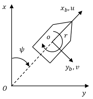
Earth-fixed and body-fixed coordinate systems
The ship maneuvering motion is described using a 3-DOF model in the horizontal plane, considering surge, sway, and yaw motions. Following the MMG standard method (Yasukawa and Yoshimura, 2015), the equations of motion in the body-fixed coordinate system are expressed as:
| (1) |
| (2) |
| (3) |
where m is the ship mass, Izz is the moment of inertia about the vertical axis, and xG is the longitudinal position of the center of gravity. u and v denote the surge and sway velocities in the body-fixed frame, and r is the yaw rate. The term , , and represent their time derivatives, respectively, while X, Y, N are the total hydrodynamic forces and moment acting on the ship.
2.2 Coordinate transformation
Voyage data recorded by the onboard measurement system contains: Latitude, Longitude, Speed Over Ground (SOG), Course Over Ground (COG), Heading (HDG), and Rate Of Turn (ROT). Latitude and Longitude are converted to Cartesian coordinates x and y in the Earth-fixed frame using the Universal Transverse Mercator (UTM) projection, providing position coordinates in meters. SOG and COG describe the magnitude and direction of the ship's velocity vector over ground, while HDG represents the direction the bow is pointing. The difference between COG and HDG arises from the effects of wind, waves, and ocean currents. The yaw rate r and heading angle ψ are directly obtained from ROT and HDG, respectively. The surge velocity u and sway velocity v are obtained by projecting the SOG vector onto the body-fixed axes as follows (Inazu et al., 2020):
| (4) |
| (5) |
2.3 EKF-based force estimation
The EKF is widely used to estimate state variables of nonlinear state-space models (Hoff, 1995). Since the algorithm is well established, only the final forms are presented here. The state vector is defined as:
| (6) |
The hydrodynamic forces X, Y, and N are modeled as third-order Gauss–Markov model. The third-order Gauss–Markov model is adopted following Yoon and Rhee (2003), where this formulation was shown to provide sufficient flexibility to represent the time-varying behavior of hydrodynamic forces.
| (7) |
where wX, wY, and wN are independent zero-mean Gaussian white noise processes.
The measurement vector consists of quantities derived from voyage data:
| (8) |
The predicted covariance, Kalman gain, filtered state vector, and error covariance matrix are given by:
| (9) |
| (10) |
| (11) |
| (12) |
where is the Jacobian of the nonlinear state transition function f. H is the Jacobian matrix of , I is the identity matrix, Q is the process noise covariance matrix, and R is the measurement noise covariance matrix. Both Q and R are assumed to be diagonal. The elements of R can be estimated from the variance of the measured data, while the elements of Q are more difficult to determine and are obtained by iterative tuning until satisfactory filter performance is achieved (Hoff, 1995).
2.4 PINN-based force estimation
PINNs incorporate physical constraints into the neural network training process through a physics-based loss function, allowing the model to learn from data while remaining consistent with the governing equations (Raissi et al., 2019). In this study, the PINN is implemented as a fully connected feedforward neural network following the formulation of Xu et al. (2022). While the EKF requires manual tuning of the noise covariance matrices Q and R, the PINN architecture is systematically determined through grid search hyperparameter optimization (Jaber et al., 2025). The search covers the number of hidden layers, neurons per layer, and activation function.
In this study, the network takes six ship state variables [u,v,r,x,y,ψ] as input and produces the three estimated hydrodynamic forces as output. The network is trained by minimizing a total loss function, which includes:
| (13) |
where λd and λp are the weights that balance the contribution of the data loss and physics loss, respectively. In this study, both weights are set to 1.0, consistent with the original PINN formulation of Raissi et al. (2019). This choice is justified by the fact that both loss terms are computed as MSE over the same dataset and share the same physical units, making their magnitudes naturally comparable (Rohrhofer et al., 2023). The total loss is minimized using the Adam optimizer. The data loss measures the difference between the PINN output and the EKF pseudo-labels:
| (14) |
where , , are the EKF pseudo-labels at time step k. The physics loss enforces consistency with Eqs. (1)–(3):
| (15) |
where Xk, Yk, Nk are the forces and moment computed from Eqs. (1)–(3) using the measured states. The time derivatives , , and are computed numerically using finite differences with a fixed time step of 0.1 s for simulation data and 1 s for voyage data.
2.5 PINE framework
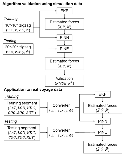
The overall PINE framework is shown in Fig. 2. The framework consists of two stages: training and testing. In the training stage, ship state variables are fed into the EKF to generate pseudo-labels , , and . These pseudo-labels, together with the ship states, are used to train the PINN by minimizing the total loss L defined in Eq. (13). The trained model is saved for use in the testing stage. In the testing stage, the trained PINN takes unseen ship state variables as input and produces the estimated hydrodynamic forces , , and as output.
Overall framework of the proposed PINE method
The framework is applied in two scenarios. In the first scenario, PINE is trained on simulation data from a 10o-10o zigzag test and tested on a 20o-20o zigzag test, where ground-truth forces are available for validation using R2 and NRMSE. Both PINE(Lp) and PINE(Lp+Ld) are evaluated to quantify the contribution of EKF pseudo-labels to training performance. Note that the EKF pseudo-labels inherently contain estimation errors due to linearization and correction of the noise covariance matrix, which are directly propagated into the training process through the data loss term Ld. While these errors may affect the training process, the physics loss term Lp simultaneously enforces consistency with the ship equations of motion, preventing the estimator from overfitting to inaccurate pseudo-labels. The 10o-10o zigzag test is selected for training because it provides sufficient excitation of the ship dynamics, while the 20o-20o zigzag test is used for testing to evaluate the generalization ability of the trained model. In the second scenario, PINE(Lp+Ld) is trained on a segment of real voyage data and tested on another segment, where no ground-truth forces are available. For real voyage data, the coordinate transformation described in Section 2.2 is applied to convert the measured quantities LAT, LON, HDG, COG, SOG, and ROT into the body-fixed state variables (u, v, r, x, y, ψ) before being fed into the EKF and PINN.
A key advantage of PINE is that the EKF provides a physically informed supervisory signal when no ground-truth force measurements are available, while the PINN produces improved estimates beyond the limitations of the EKF alone. Once trained, the model can be deployed directly on a ship's onboard system for real-time estimation without retraining, and can be fine-tuned for other ships using transfer learning (Pan and Yang, 2010).
3. Simulation validation
The simulation dataset is generated by numerically solving the MMG standard equations of motion (Yasukawa and Yoshimura, 2015) in three degrees of freedom, with hydrodynamic forces decomposed into hull, propeller, and rudder contributions. The hydrodynamic coefficients are taken from Nguyen et al. (2022), estimated through captive model tests in a towing tank. All simulations are performed at full scale for the Korea Autonomous Surface Ship (KASS) at its design speed of 15.5 kn. The principal particulars of KASS are listed in Table 1.

Principal particulars of KASS
Two maneuvering scenarios are considered: the 10o-10o and 20o-20o zigzag tests, and the corresponding simulated ship states are shown in Fig. 3. The 10o-10o zigzag dataset is used for EKF-based force estimation, hyperparameter optimization, and PINN training because it best represents the typical dynamic range of a large ship during voyage. This dataset is divided into a training set (75%) and a validation set (25%) in chronological order to preserve the temporal structure of the data and avoid data leakage. The 20o-20o zigzag dataset is used to assess the generalizability of the trained model because it involves larger rudder angles that were not encountered during training.
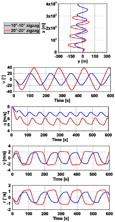
Simulated ship states for 10o-10o and 20o-20o zigzag tests
The EKF is applied to the 10o-10o zigzag data to generate pseudo-labels. Fig. 4 shows the estimated hydrodynamic forces , , and from the EKF compared against the simulation ground truth for the 10o-10o zigzag test. The EKF achieves reasonable accuracy for and , with R2 of 0.976 and 0.948 and NRMSE of 0.156 and 0.227, respectively. However, the estimation of remains limited, with R2 of 0.572 and NRMSE of 0.652. Despite this limitation, the EKF estimates are used as pseudo-labels for PINE(Lp+Ld) training, where the combined loss helps reduce the effect of linearization errors through physics-constrained learning. In addition, since the PINN takes the directly measured ship states (u, v, r, x, y, ψ) as input, the coupling between force components through the drift angle is correctly preserved regardless of EKF estimation accuracy.
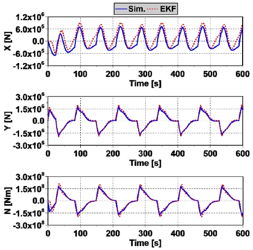
Hydrodynamic force estimation for 10o-10o zigzag
A grid search is performed to identify the optimal PINN architecture (Jaber et al., 2025). The search covers the number of epochs {500, 1000, 1500, 2000, 2500, 3000}, hidden layers {1, 2, 3, 4, 5}, neurons per layer {3, 6, 9, 12, 15}, and activation functions {linear, tanh, ReLU, sigmoid}. For each configuration, the average NRMSE across the three force components , , and is computed on the validation set as the selection criterion. Table 2 summarizes selected representative results, chosen to illustrate the individual effect of each hyperparameter while holding the others fixed. The optimal architecture consists of 5 hidden layers, 15 neurons per layer, tanh activation, and 3000 epochs, yielding the lowest average NRMSE and is therefore adopted for all subsequent training.
PINE architecture optimization for simulation data
Using the optimal configuration, two training configurations are compared as an ablation study: PINE(Lp), which minimizes only the physics loss, and PINE(Lp+Ld), which minimizes the combined loss as defined in Eq. (13). In both configurations, the EKF is applied to generate pseudo-labels, the distinction lies solely in whether these pseudo-labels are incorporated as supervised training targets in the loss function. The training loss for each configuration is computed as the RMSE between the predicted and ground-truth hydrodynamic forces on the validation set. Fig. 5 shows the training loss convergence for both configurations. At epoch 3000, PINE(Lp) achieves a final loss of 1.112×10⁻² while PINE(Lp+Ld) reaches 2.063×10⁻³. The latter converges faster and to a lower final value, indicating that directly incorporating EKF pseudo-labels into the loss function effectively accelerates and stabilizes training.
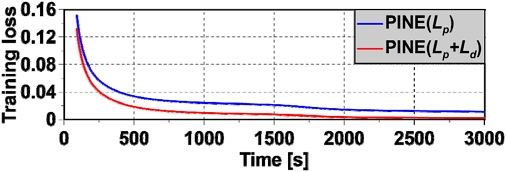
Training loss for simulation data
The trained models are then applied directly to the 20o-20o zigzag ship states without retraining. Fig. 6 shows the estimated hydrodynamic forces from EKF, PINE(Lp), and PINE(Lp+Ld) compared to the simulation ground truth. The EKF produces good estimates for and , but shows larger errors for . PINE(Lp) produces accurate estimates for all three force components. PINE(Lp+Ld) further improves upon both methods and produces the closest agreement with the ground truth across all force components. Table 3 provides a quantitative comparison. PINE(Lp+Ld) achieves the highest R2 and the lowest NRMSE for all force components. The most notable improvement is observed for , where R2 increases from 0.820 for EKF and 0.951 for PINE(Lp) to 0.997, while NRMSE reduces from 0.423 and 0.220 to 0.053. For and , all three methods perform well, but PINE(Lp+Ld) still achieves further improvement.
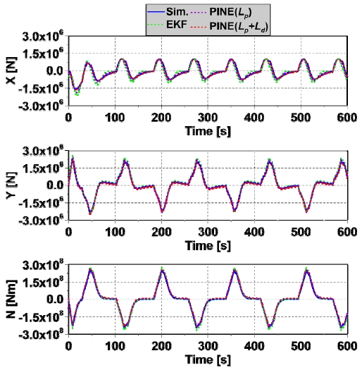
Hydrodynamic force estimation for 20o-20o zigzag
Hydrodynamic force estimation performance for 20o-20o zigzag
The advantage of PINE(Lp+Ld) becomes more important when applied to real voyage data, where no ground-truth force measurements are available. In this case, PINE(Lp) relies solely on the physics loss and receives no data-driven supervision, which limits its reliability. By contrast, PINE(Lp+Ld) leverages EKF pseudo-labels as a supervisory signal, enabling stable and accurate training even without ground-truth measurements. For this reason, only PINE(Lp+Ld) is applied in the real voyage data application.
4. Application to Voyage data
The voyage data used in this study were recorded by the onboard measurement system of KASS during a voyage from the Incheon area to the Busan area along the western and southern coast of Korea. The data spans from 2025-05-17 to 2025-05-20, with a total duration of approximately 66 hours and a sampling interval of 1 second. The training and testing segments are selected based on data quality and continuity, prioritizing periods with stable sensor recordings and sufficient maneuver variation. The training segment spans 2025-05-17 22:30 to 2025-05-18 10:50 (approximately 12.3 hours), and the testing segment spans 2025-05-18 13:23 to 2025-05-19 04:10 (approximately 14.8 hours). A gap of approximately 2.5 hours between the two segments, during which the data logging system was temporarily interrupted, was excluded from the analysis. The coordinate transformation described in Section 2.2 is applied to convert the measured quantities LAT, LON, HDG, COG, SOG, and ROT into the body-fixed state variables (u, v, r, x, y, ψ). The transformed state variables for both the training and testing segments are shown in Fig. 7.
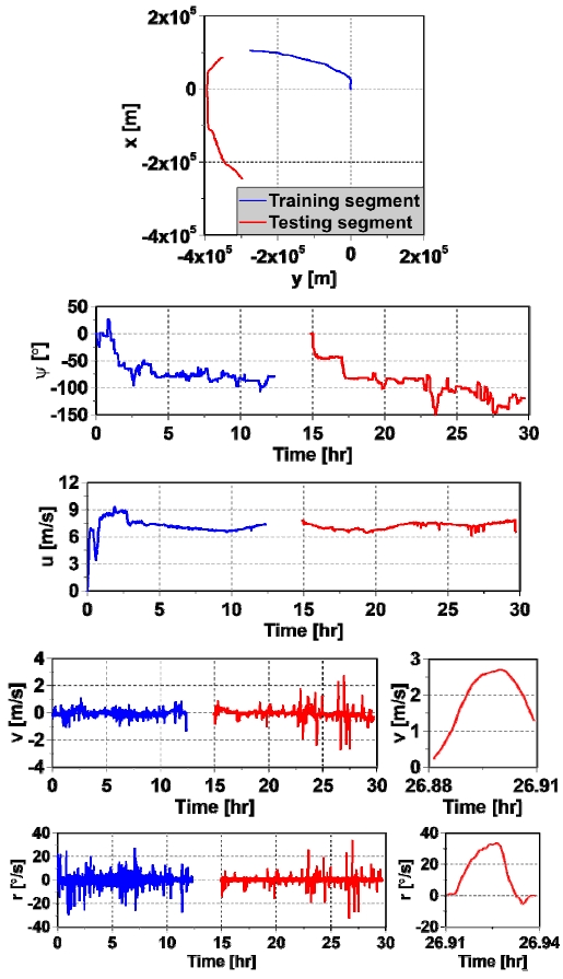
Transformed ship states for voyage data
Although v and r in Fig. 7 appear noisy due to the compression of approximately 30 hours of data into a single figure, the fluctuations reflect real physical variations caused by continuous rudder adjustments rather than measurement noise. As shown in the insets, both data vary smoothly at the sampling time of 1 second. Therefore, the finite difference approximations of , , and represent actual ship accelerations, and the resulting forces Xk, Yk, and Nk computed from Eqs. (1)–(3) provide physically meaningful constraints for the physics loss term Lp in Eq. (15).
The EKF is applied to the training segment to generate pseudo-labels , , and . Since no ground-truth force measurements are available for real voyage data, the quality of the EKF estimates cannot be directly evaluated. However, as demonstrated in the simulation validation in Section 3, the EKF provides reasonable force estimates that serve as an effective supervisory signal for PINE(Lp+Ld) training, with the physics loss independently compensating for linearization errors.
A grid search is performed to identify the optimal PINN architecture for the voyage data, following the same procedure as in Section 3, with neurons per layer extended to {16, 32, 64, 128, 256} to account for the increased complexity of real voyage data. Since no ground-truth forces are available, the validation loss is computed as the sum of the data loss and physics loss on a validation data (25%) of the training segment. Table 4 presents selected representative results. The optimal architecture consists of 3 hidden layers, 32 neurons per layer, tanh activation, and 3000 epochs, yielding the lowest validation loss.
PINE architecture optimization for voyage data
Using the optimal configuration, the training loss convergence of PINE(Lp+Ld) is shown in Fig. 8. The model converges steadily and reaches a low final validation loss at epoch 3000, consistent with the simulation results in Section 3. This confirms that EKF pseudo-labels provide an effective supervisory signal for PINN training even when no ground-truth force measurements are available.
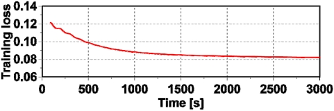
Training loss for voyage data
The trained PINE(Lp+Ld) model is applied to the testing segment to estimate the hydrodynamic forces. The results are shown in Fig. 9, alongside the EKF estimates for comparison. Although ground-truth force measurements are unavailable for direct validation, several observations can be made. For , both methods produce positive estimates consistent with the resistive nature of surge force during forward motion. After hour 8 of the testing segment (corresponding to hour 23 of the full voyage record in Fig. 7), ψ changes from –90o to –150o (counterclockwise), inducing a negative yaw rate r of approximately –10o/s and larger oscillations in v of approximately 2 m/s while u remains stable at approximately 7 m/s. Since is approximately zero, Eq. (1) gives , where the term -vr becomes positive with r < 0, explaining the upward drift in estimated by PINE(Lp+Ld). For , the dominant term ur in Eq. (2) becomes negative with u > 0 and r < 0, explaining the opposing downward drift observed in both PINE(Lp+Ld) and EKF estimates. For , both methods produce estimates that oscillate around zero throughout the testing segment, consistent with the periodic nature of yaw motion during a long-distance voyage. Overall, PINE(Lp+Ld) captures the general trends of all three force components, demonstrating its practical applicability for hydrodynamic force estimation from real voyage data.
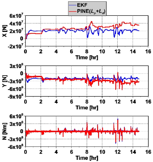
Hydrodynamic force estimation for testing segment
5. Conclusion
This paper proposed PINE, a Physics-Informed Neural Estimator that integrates the EKF and PINN for hydrodynamic force estimation from voyage data. The EKF generates pseudo-labels as supervised training targets, while the physics loss independently enforces consistency with the ship equations of motion through automatic differentiation.
Validation on simulation data demonstrated that PINE(Lp+Ld) consistently outperforms both the standalone EKF and PINE(Lp) across all three force components. For the 20o-20o zigzag generalization test, PINE(Lp+Ld) achieved R2 of 0.997, 0.997, and 0.996 with NRMSE of 0.053, 0.050, and 0.062 for surge force, sway force, and yaw moment, respectively. The framework was further applied to real voyage data from KASS, where the estimated forces capture the general trends of all three force components, confirming its practical applicability without requiring dedicated sea trial maneuvers or ground-truth force measurements.
The current study has several limitations. First, the framework is validated on a single ship type (KASS) and a limited set of maneuvers. Second, the EKF requires manual tuning of Q and R, which may affect pseudo-label quality. Third, environmental disturbances such as wind, waves, and ocean currents are not accounted for, which may introduce bias in the velocity estimates from COG and SOG data. Fourth, periodic model updating may be necessary for long-duration deployments. Future work will address these limitations by extending the framework to additional ship types, incorporating automatic noise tuning, integrating environmental disturbance models, performing indirect validation of the estimated forces through hydrodynamic coefficient identification, and conducting a quantitative comparison with the MBF smoother to characterize the trade-off between real-time capability and batch estimation accuracy. In addition, more efficient hyperparameter tuning approaches beyond grid search will be investigated.
Acknowledgments
This research was supported by the 'Development of Autonomous Ship Technology(PJT201313, Development of Autonomous Navigation System with Intelligent Route Planning Function, 50%)' funded by the Ministry of Oceans and Fisheries(MOF, Korea) and by the Institute of Information & Communications Technology Planning & Evaluation(IITP)-Innovative Human Resource Development for Local Intellectualization program grant funded by the Korea government(MSIT) (IITP-2026-RS-2024-00436773, 50%).
References
-
Choi, H., Kim, D.J., Kim, Y.G., Yeo, D.J., Yun, K. and Lee, G., 2022. A study on the captive model test of KCS in regular waves. Journal of the Society of Naval Architects of Korea, 59(5), pp.296-305.
[https://doi.org/10.3744/SNAK.2022.59.5.296]

-
Fossen, T.I., 2011. Handbook of marine craft hydrodynamics and motion control. John Wiley & Sons, Chichester, UK.
[https://doi.org/10.1002/9781119994138]
- Hoff, J.C., 1995. Aircraft parameter estimation by estimation-before-modelling technique. PhD Thesis. Cranfield: Cranfield University.
-
Inazu, D., Ikeya, T., Iseki, T. and Waseda, T., 2020. Extracting clearer tsunami currents from shipborne automatic identification system data using ship yaw and equation of ship response. Earth, Planets and Space, 72(1), 41.
[https://doi.org/10.1186/s40623-020-01165-7]
-
Jaber, Y., Dharmasena, P., Nassif, A. and Nassif, N., 2025. Hyperparameter optimization of neural networks using grid search for predicting HVAC heating coil performance. Buildings, 15(15), 2753.
[https://doi.org/10.3390/buildings15152753]
-
Jeon, M.J., Yoon, H.K., Ryu, J.K., Lee, W.H. and Ku, P.M., 2021. Evaluation of maneuverability in still water of an unmanned surface vehicle through sea trials. Journal of the Society of Naval Architects of Korea, 58(4), pp.253-261.
[https://doi.org/10.3744/SNAK.2021.58.4.253]
-
Li, H., Jiao, H. and Yang, Z., 2023. AIS data-driven ship trajectory prediction modelling and analysis based on machine learning and deep learning methods. Transportation Research Part E: Logistics and Transportation Review, 175, 103152.
[https://doi.org/10.1016/j.tre.2023.103152]
-
Mai, T.L., Vo, A.K. and Yoon, H.K., 2022. Study on pure roll test of a ship using CFD simulation. Journal of the Society of Naval Architects of Korea, 59(6), pp.338-344.
[https://doi.org/10.3744/SNAK.2022.59.6.338]
- Nguyen, T.T.D., Mai, V.T., Lee, S. and Yoon, H.K., 2022. An experimental study on hydrodynamic forces of Korea autonomous surface ship in various loading conditions. Journal of Navigation and Port Research, 46(2), pp.73-81.
-
Pan, S.J. and Yang, Q., 2010. A survey on transfer learning. IEEE Transactions on Knowledge and Data Engineering, 22(10), pp.1345-1359.
[https://doi.org/10.1109/TKDE.2009.191]
-
Park, J., Rhee, S.H., Lee, S., Yoon, H.K., Seo, J., Lee, P.Y., Kim, H.S. and Lee, H., 2020. Study on the estimation of autonomous underwater vehicle’s maneuverability using vertical planar motion mechanism test in self-propelled condition. Journal of the Society of Naval Architects of Korea, 57(5), pp.287-296.
[https://doi.org/10.3744/SNAK.2020.57.5.287]
-
Park, J.Y. and Lee, J.H., 2020. A study on full-scale maneuvering trials using bow thruster. Journal of the Society of Naval Architects of Korea, 57(1), pp.52-59.
[https://doi.org/10.3744/SNAK.2020.57.1.052]
-
Raissi, M., Perdikaris, P. and Karniadakis, G.E., 2019. Physics-informed neural networks: a deep learning framework for solving forward and inverse problems involving nonlinear partial differential equations. Journal of Computational Physics, 378, pp.686-707.
[https://doi.org/10.1016/j.jcp.2018.10.045]
-
Rohrhofer, F.M., Posch, S., Gößnitzer, C. and Geiger, B.C., 2023. Data vs. physics: the apparent Pareto front of physics-informed neural networks. IEEE Access, 11, pp.118596-118607.
[https://doi.org/10.1109/ACCESS.2023.3302892]
-
Terziev, M., Tezdogan, T. and Incecik, A., 2022. Scale effects and full-scale ship hydrodynamics: a review. Ocean Engineering, 245, 110496.
[https://doi.org/10.1016/j.oceaneng.2021.110496]
-
Xia, G., Zhou, Z., Han, F., Peng, X., Zhao, W., Wu, Y. and Lin, Q., 2024. Real-time digital twin of autonomous ships based on virtual-physical mapping model. Physics of Fluids, 36(8), 087109.
[https://doi.org/10.1063/5.0222332]
-
Xu, P.F., Han, C.B., Cheng, H.X., Cheng, C. and Ge, T., 2022. A physics-informed neural network for the prediction of unmanned surface vehicle dynamics. Journal of Marine Science and Engineering, 10(2), 148.
[https://doi.org/10.3390/jmse10020148]
-
Yasukawa, H. and Yoshimura, Y., 2015. Introduction of MMG standard method for ship maneuvering predictions. Journal of Marine Science and Technology, 20, pp.37-52.
[https://doi.org/10.1007/s00773-014-0293-y]
-
Yoon, H.K. and Rhee, K.P., 2003. Identification of hydrodynamic coefficients in ship maneuvering equations of motion by estimation-before-modeling technique. Ocean Engineering, 30(18), pp.2379-2404.
[https://doi.org/10.1016/S0029-8018(03)00106-9]
-
You, Y., 2019. Different approaches for estimating the full-scale performance of a ship based on 3-DOF maneuvering equations of motion: given speed, RPM or power. Journal of the Society of Naval Architects of Korea, 56(5), pp.427-438.
[https://doi.org/10.3744/SNAK.2019.56.5.427]
-
Zhang, M., Taimuri, G., Zhang, J. and Hirdaris, S., 2023. A deep learning method for the prediction of 6-DoF ship motions in real conditions. Proceedings of the Institution of Mechanical Engineers, Part M: Journal of Engineering for the Maritime Environment, 237(4), pp.887-905.
[https://doi.org/10.1177/14750902231157852]
Hoang Thien Vu: Conceptualization, Formal analysis, Funding acquisition, Investigation, Methodology, Writing – original draft; Jeonghong Park: Data curation, Project administration, Supervision; Hyeon Kyu Yoon: Conceptualization, Project administration, Supervision, Validation, Writing – review & editing.